Fits a power-law component of the model: $$y(f) = \frac{\mu}{\beta n} \frac{1}{f^2}$$ where \( \mu/\beta \) is the mutation rate per effective cell division, and n is the number of bins in the spectrum. The power-law exponent of this model equals 2, as expected by Williams et al. (2016) and Durrett (2013). This model is valid under the assumptions of exponential population growth, constant mutation rate, and absence of selectively advantageous micro-clones desctibed by Tung and Durrett (2021).
Usage
fit_powerlaw_tail_fixed(object, ...)

# S3 method for cevodata
fit_powerlaw_tail_fixed(
  object,
  rsq_treshold = 0.98,
  lm_length = 0.05,
  name = "powerlaw_fixed",
  pct_left = 0.05,
  pct_right = 0.95,
  verbose = get_cevomod_verbosity(),
  ...
)

layer_lm_fits(cd, model_name = "powerlaw_fixed", ...)
Arguments
- object
SNVs tibble object
- ...
other params passed to geom_segment()
- rsq_treshold
R-squared tresholds to keep model as neutral
- lm_length
length of the linear model fits
- name
name in the models' slot
- pct_left
drop pct of the lowerst frequency variants to improve fit
- pct_right
drop pct of the highest frequency variants to improve fit
- verbose
verbose?
- cd
cevodata
- model_name
modelname
Details
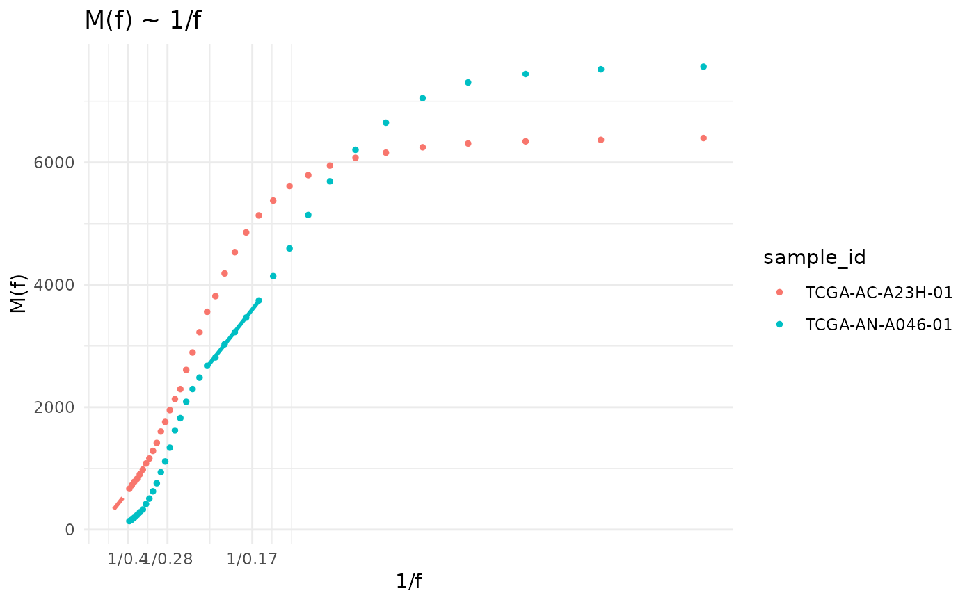
This model is fitted using the statistic $$M(f) = \frac{\mu}{\beta} \frac{1}{f}$$ described by Williams et al. (2016). Using the equations described in Williams et al. (2018) evolutionary parameters of detected subclones can be calculated.
Examples
data("tcga_brca_test")
snvs <- SNVs(tcga_brca_test) |>
  dplyr::filter(sample_id %in% c("TCGA-AC-A23H-01","TCGA-AN-A046-01"))

cd <- init_cevodata("Test") |>
  add_SNV_data(snvs) |>
  intervalize_mutation_frequencies() |>
  calc_Mf_1f() |>
  calc_SFS() |>
  fit_powerlaw_tail_fixed(rsq_treshold = 0.99)
#> Calculating f intervals, using VAF column
#> Calculating Williams's M(f) ~ 1/f statistics, using VAF column
#> Calculating SFS statistics
#> Fitting williams neutral models...

plot(cd$models$Mf_1f, from = 0.05, to = 0.4, scale = FALSE) +
  layer_lm_fits(cd)