Nice extention of the default ggplot2 stats. However, it should be easier to use the plot_cumulative_tails() function.
Usage
stat_cumulative_tail(
  mapping = NULL,
  data = NULL,
  geom = "point",
  position = "identity",
  na.rm = FALSE,
  show.legend = NA,
  inherit.aes = TRUE,
  bins = 100,
  ...
)
Arguments
- mapping
Set of aesthetic mappings created by
aes(). If specified andinherit.aes = TRUE(the default), it is combined with the default mapping at the top level of the plot. You must supplymappingif there is no plot mapping.- data
The data to be displayed in this layer. There are three options:
If
NULL, the default, the data is inherited from the plot data as specified in the call toggplot().A
data.frame, or other object, will override the plot data. All objects will be fortified to produce a data frame. Seefortify()for which variables will be created.A
functionwill be called with a single argument, the plot data. The return value must be adata.frame, and will be used as the layer data. Afunctioncan be created from aformula(e.g.~ head(.x, 10)).- geom
geom
- position
Position adjustment, either as a string naming the adjustment (e.g.
"jitter"to useposition_jitter), or the result of a call to a position adjustment function. Use the latter if you need to change the settings of the adjustment.- na.rm
If
FALSE, the default, missing values are removed with a warning. IfTRUE, missing values are silently removed.- show.legend
logical. Should this layer be included in the legends?
NA, the default, includes if any aesthetics are mapped.FALSEnever includes, andTRUEalways includes. It can also be a named logical vector to finely select the aesthetics to display.- inherit.aes
If
FALSE, overrides the default aesthetics, rather than combining with them. This is most useful for helper functions that define both data and aesthetics and shouldn't inherit behaviour from the default plot specification, e.g.borders().- bins
number of bins
- ...
Other arguments passed on to
layer(). These are often aesthetics, used to set an aesthetic to a fixed value, likecolour = "red"orsize = 3. They may also be parameters to the paired geom/stat.
Details
stat_bin() is suitable only for continuous x data. If your x data is
discrete, you probably want to use stat_count().
By default, the underlying computation (stat_bin()) uses 30 bins;
this is not a good default, but the idea is to get you experimenting with
different number of bins. You can also experiment modifying the binwidth with
center or boundary arguments. binwidth overrides bins so you should do
one change at a time. You may need to look at a few options to uncover
the full story behind your data.
In addition to geom_histogram(), you can create a histogram plot by using
scale_x_binned() with geom_bar(). This method by default plots tick marks
in between each bar.
Orientation
This geom treats each axis differently and, thus, can thus have two orientations. Often the orientation is easy to deduce from a combination of the given mappings and the types of positional scales in use. Thus, ggplot2 will by default try to guess which orientation the layer should have. Under rare circumstances, the orientation is ambiguous and guessing may fail. In that case the orientation can be specified directly using the orientation parameter, which can be either "x" or "y". The value gives the axis that the geom should run along, "x" being the default orientation you would expect for the geom.
Aesthetics
geom_histogram() uses the same aesthetics as geom_bar();
geom_freqpoly() uses the same aesthetics as geom_line().
Computed variables
These are calculated by the 'stat' part of layers and can be accessed with delayed evaluation.
after_stat(count)
number of points in bin.after_stat(density)
density of points in bin, scaled to integrate to 1.after_stat(ncount)
count, scaled to a maximum of 1.after_stat(ndensity)
density, scaled to a maximum of 1.after_stat(width)
widths of bins.
Dropped variables
weightAfter binning, weights of individual data points (if supplied) are no longer available.
See also
stat_count(), which counts the number of cases at each x
position, without binning. It is suitable for both discrete and continuous
x data, whereas stat_bin() is suitable only for continuous x data.
Examples
library(ggplot2)
data("tcga_brca_test")
snvs <- SNVs(tcga_brca_test)

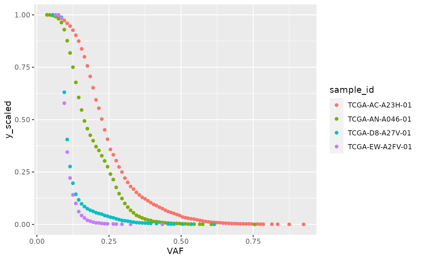
ggplot(snvs, aes(VAF, color = sample_id)) +
 stat_cumulative_tail()


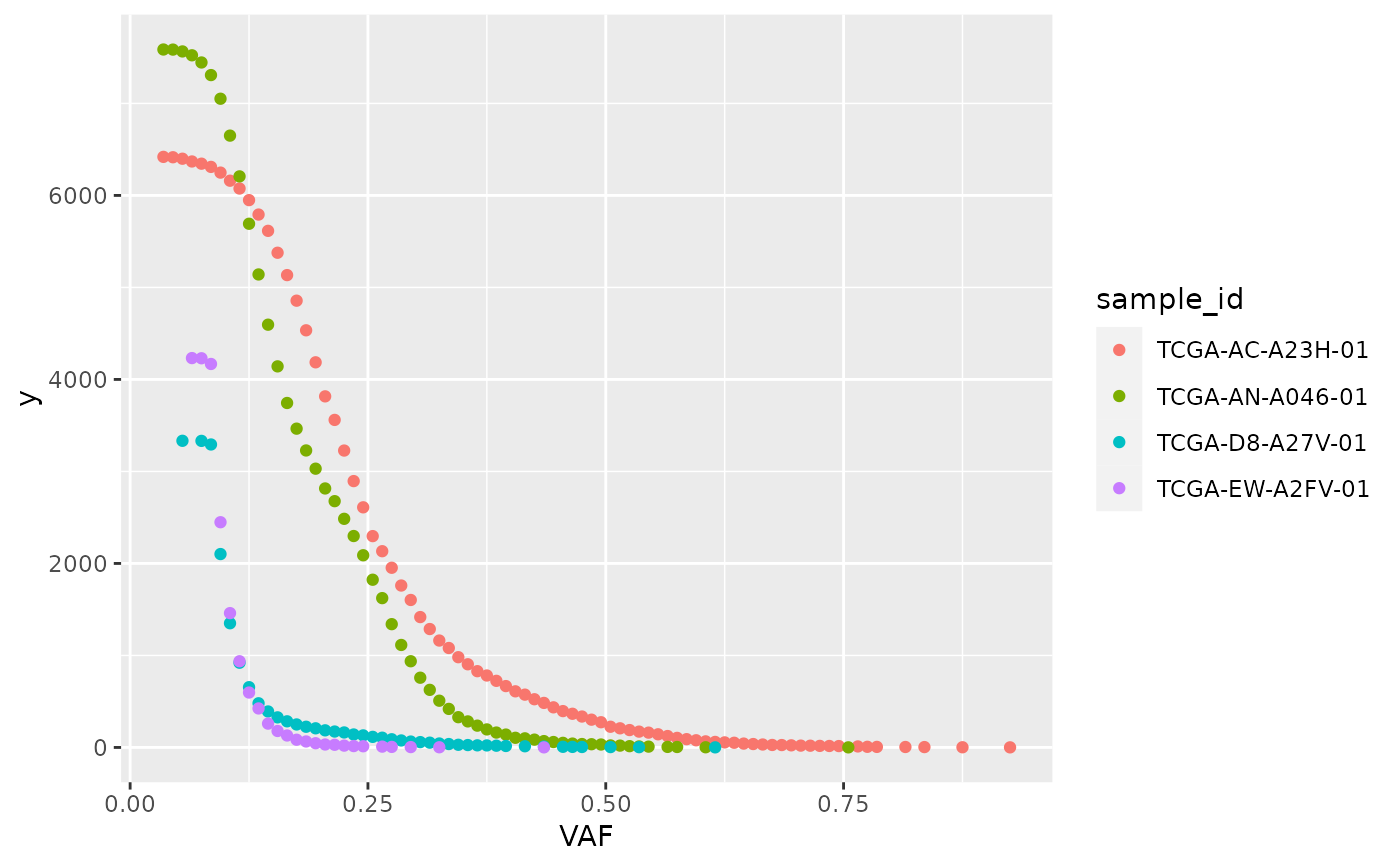
ggplot(snvs, aes(VAF, y = stat(y), color = sample_id)) +
 stat_cumulative_tail()
#> Warning: `stat(y)` was deprecated in ggplot2 3.4.0.
#> ℹ Please use `after_stat(y)` instead.

